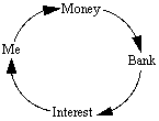
Figure 1
Models are the things we build to help us understand things
better. When dealing with concepts of reality we have as the only
alternative those abstractions we develop as models, or in situations
where it is simply to costly to build the real thing, we build
models to help us understand. In short models are simplifications,
or abstractions, of reality intended to promote understanding.
Whether the models we create are good models or poor models depends
on the extent to which they aid us in developing the understanding
we seek. As to whether a model is correct or incorrect is probably
something which will only become evident in time.
The difficulty, or I should say limiting characteristic, of most
of the models we build is that they are static in nature. That
is, they are models that represent a snapshot of something at
a particular point in time. Yet, reality is not static. Reality
is constantly changing through our interactions with it, and the
interactions between all of its parts, reality is dynamic in its
nature. The question arises as to how we can believe that it is
possible to build static models of dynamic reality and expect
them to aid our understanding to anything more than a very limited
extent.
The answer to this question is provided by something call Dynamic
Modeling, or as it was probably better known in a prior incarnation,
Simulation. Reality operates "in" time, real time. Dynamic
Modeling operates "on" time, serving to compress it
in such a way that it provides us with a view of the evolution
of our constructions through time.
As an example consider the interpretation we have of a bank savings
account. We know that if we put money in our savings account the
bank will periodically pay us interest on the money in the account.
This may be represented by the following very simple model.

This diagram, a very simplistic model, says if I give Money
to the Bank then the Bank will give Interest to Me. Pretty simple,
yes? Yet what does this model tell us about how things change
over time? Not much.
Now consider the following diagram.

This is what is typically called a Systems Thinking, or Causal
Loop, Diagram. The intent is to add a bit more information than
is found in Figure 1. If you're not familiar with these diagrams
don't let it get to you. They're not as difficult to read as you
might think. For addition information on reading diagrams see:
Introduction to Systems Thinking.
What the diagram indicates is simply influences between various
parts of the system, with indicators as to the nature of the influence
being either the same (S) or opposite (O).
Figure 2 reads as follows: Money and Interest both serve to increase
the Principal. Principal, acting in conjunction with Interest
Rate, both serve to increase Interest. This Interest then feeds
into Principal serving to increase it even more. The snowball
rolling down hill at the center of the diagram indicates this
is a reinforcing structure, reinforcing in that it feeds upon
itself.
Figure 2 gives some additional information over what was provided
in Figure 1. Some additional information in terms of how the parts
of the system influence each other, yet Figure 2 still gives us
little information about how the system operates "in"
time.
Suppose we consider the following scenario. If I put $100 in the
bank and the bank pays an interest of 6% quarterly, how much money
will I have in 8 years? Yes, there is a mathematical formula by
which you can calculate this. In most dynamic systems the formulas
are of such complexity as to become completely unmanageable.
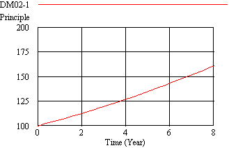
Figure 3 is the result of associating, or embedding, equations
into the model and running it with quarterly calculations. As
a result, the model indicates you would have $161.03 at the end
of the 8th year.
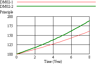
Now suppose the bank was paying 8% interest as opposed to 6%.
How would this change the result? This is presented in Figure
4, which compares the result with Figure 3. This would result
in $188.45 at the end of 8 years.
Now suppose I also put another $10 in the account every quarter.
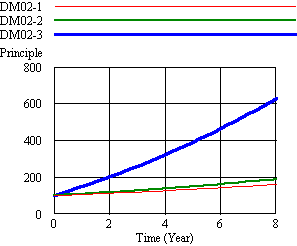
Figure 5 indicates that simply adding $10 a quarter to the
account will produce $630.72 at the end of 8 years. A substantial
increase, when compared with the result of Figure 3 and Figure
4, for a small ongoing addition to the principal.
In each of these examples the static model of the system has not
changed, yet the dynamic result is markedly different in each
of the examples cited.
Now let's consider an example which isn't quite as simplistic
as the Interest and Principal one.
Consider a rather high profile consulting company with 120 employees.
Of these 120 employees 60 are professionals and 60 are rookies
in training to be professionals. The company bills their clients
at a rate of $15k per month for professionals and $5k per month
for rookies. Also, it takes 6 months to train a rookie to be a
professional. Currently the company wants to remain at 120 employees,
and since there are 5 professionals that quit each month, the
company hires a new rookie for each professional that quits. Figure
6 is a systems thinking diagram of this description.
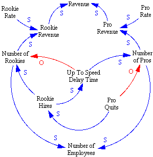
The overall result of this system is that it is in a steady
state. The 120 employees of this company will generate $1.2 million
a month in revenue, if they're all on billing, which I understand
is a somewhat far fetched assumption.
Now, what happens if the Pro Quits rate jumps from 5 to 7 per
month beginning in the 4th month? I don't think you're going to
find a straight forward mathematical formula which will provide
an indication of the implications of this change in the system
operation. Plugging this change into the model in Figure 6 and
running the simulation produces the following operational changes
in the system.
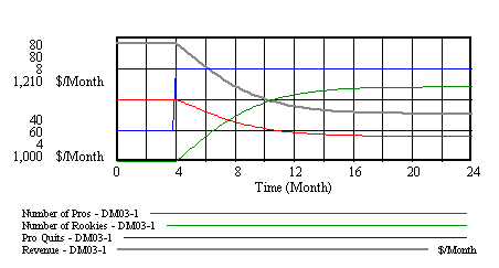
What Figure 7 portrays is that in month 4 Pro Quits jumps from
5 to 7. This one time change sets off a 12 month transition in
the system where the number of Pros declines from 60 to 48 and
the number of Rookies increases from 60 to 72. While this transition
is in progress revenue drops accordingly from $1.2 M per month
to $1.08 M.
This example should provide a foundation for the value of Dynamic
Modeling in terms of providing a capability for seeing the time
compression of reality.